Liam's Blog


  • Home

  • Archives

  • Tags

  • Categories

  • Photos

  • About

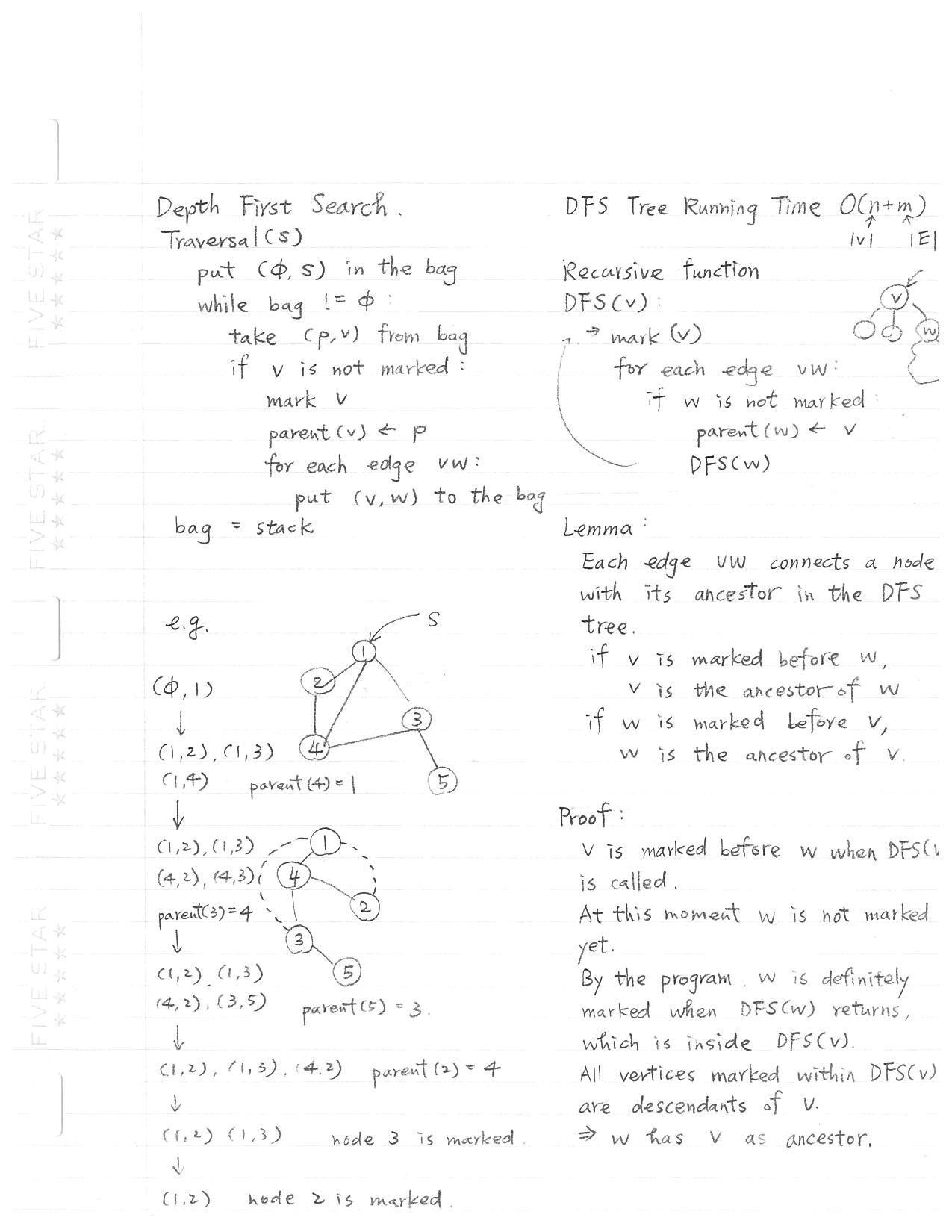
Analysis of Algorithms Lecture 3

Posted on 2018-09-27 | Post modified 2018-09-27 | In Algorithms , Basic Concepts , Graph , Depth-first Search , Directed Acyclic Graph , Weighted Graph
Read more »

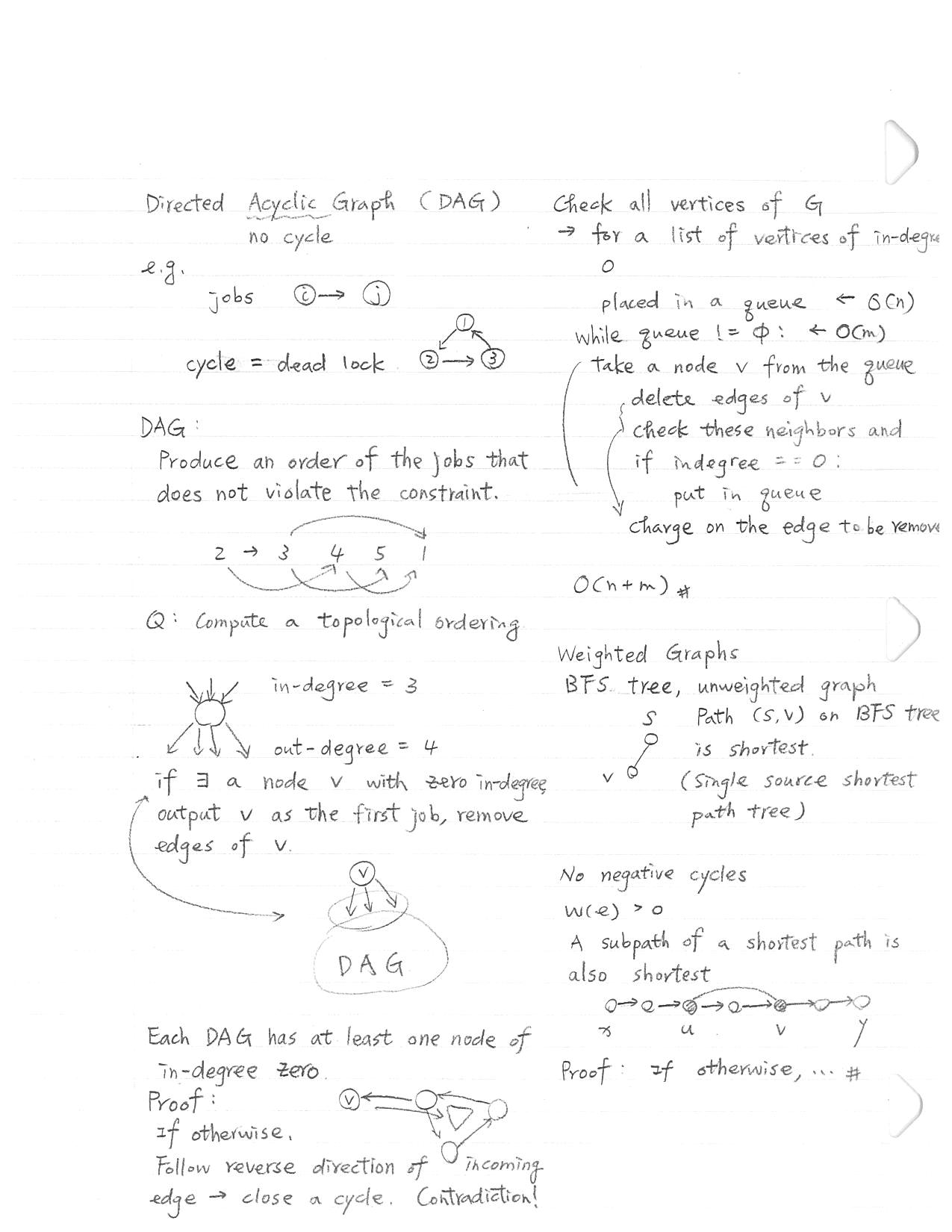
Analysis of Algorithms Lecture 2

Posted on 2018-09-27 | Post modified 2018-09-27 | In Algorithms , Basic Concepts , Graph , Graph Traversal , Tree
Read more »

Statistical Distributions

Posted on 2018-09-27 | Post modified 2018-10-11 | In Data Science

Statistics and Data Science

“A data scientist is someone who knows more statistics than a computer scientist and more computer science than a statistician.” - Josh Blumenstock (University of Washington)

Read more »

Scores and Rankings

Posted on 2018-09-26 | Post modified 2018-10-25 | In Data Science

Scores and Rankings

Scoring functions are measures that reduce multi-dimensional data to a single value, to highlight some particular property.

Rankings order items, usually by sorting scores.

Read more »

LeetCode #461 Hamming Distance

Posted on 2018-09-25 | Post modified 2018-09-27 | In Languages , LeetCode , Python , Difficulties , Easy

Problem

The Hamming distance between two integers is the number of positions at which the corresponding bits are different.

Given two integers x and y, calculate the Hamming distance.

Note

0 ≤ x, y < 231.

Example

1
2
3
4
5
6
7
8
9
10
Input: x = 1, y = 4

Output: 2

Explanation:
1 (0 0 0 1)
4 (0 1 0 0)
↑ ↑

The above arrows point to positions where the corresponding bits are different.
Read more »

Computing-with-Logic-Notes(Structures Lists Difference Lists) Part4

Posted on 2018-09-24 | Post modified 2018-09-30 | In Languages , Prolog , Conditional Evaluation

Conditional Evaluation

  • Conditional operator (the if-then-else construct in Prolog):

    • if A then B else C is written as (A -> B ; C)

      • To Prolog this means:

        Try A.

        If you can prove it, go on to prove B and ignore C.

        If A fails, however, go on to prove C ignoring B.

        e.g.

        1
        2
        3
        4
        5
        max(X, Y, Z) :-
        ( X =< Y
        -> Z = Y
        ; Z = X
        ).
  • Consider the computation of n! (i.e. the factorial of n)

    ​ factorial(N, F) :- …

    • N is the input parameter; and F is the output parameter.

    • The body of the rule species how the output is related to the input.

      • For factorial, there are two cases:

        N <= 0 and N > 0

        • if N <= 0, then F = 1
        • if N > 0, then F = N * factorial(N-1)
        1
        2
        3
        4
        5
        6
        7
        factorial(N, F) :-
        (N > 0
        -> N1 is N - 1,
        factorial(N1, F1),
        F is N * F1
        ; F = 1
        ).

Imperative Features

  • Other imperative features:

    we can think of prolog rules as imperative programs with backtracking

    1
    2
    3
    4
    5
    6
    7
    8
    program :-
    member(X, [1, 2, 3, 4]),
    write(X),
    nl,
    fail;
    true.

    ?- program. % prints all solutions
  • fail: always fails, causes backtracking.

  • !: the cut operator, prevents other rules from matching.

Arithmetic Operators

  • Integer/Floating Point operators:

    • +
    • -
    • *
    • /
    • Automatic detection of Integer/Floating Point
  • Interger operator:

    • mod
    • // (integer division)
  • Comparison operators:

    • <
    • >
    • =<
    • >=
    • Expr1 =:= Expr2 (succeeds if expression Expr1 evaluates to a number equal to Expr2)
    • Expr1 =\= Expr2 (succeeds if expression Expr1 evaluates to a number non-equal to Expr2)

Programming with Lists

  • quicksort:

    1
    2
    3
    4
    5
    6
    7
    8
    9
    10
    11
    12
    13
    14
    15
    quicksort([], []).
    quicksort([X0 | Xs], Ys) :-
    partition(X0, Xs, Ls, Gs),
    quicksort(Ls, Ys1),
    quicksort(Gs, Ys2),
    append(Ys1, [X0 | Ys2], Ys).

    partition(Pivot, [], [], []).
    partition(Pivot, [X|Xs], [X|Ys], Zs) :-
    X <= Pivot,
    % can add a '!', for cut
    partition(Pivot, Xs, Ys, Zs).
    partition(Pivot, [X|Xs], Ys, [X|Zs]) :-
    x > Pivot,
    partition(Pivot, Xs, Ys, Zs).
  • We want to define delete/3, to remove a given element from a list (called select/3 in XSB’s basic library)

    • delete(2, [1, 2, 3], X) should succeed with X = [1, 3]

    • delete(X, [1, 2, 3], [1, 3]) should succeed with X = 2

    • delete(2, X, [1, 3]) should succeed with X = [2, 1, 3]; X = [1, 2, 3]; X = [1, 3, 2]; fail

    • Algorithm:

      • When X is selected from [X | Ys], Ys results.
      • When X is selected from the tail of [H | Ys], [H | Zs] results, where Zs is the result of taking X out of Ys.
      • The program:
      1
      2
      3
      4
      delete(X, [], _) :- fail. % not needed
      delete(X, [X | Ys], Ys).
      delete(X, [Y | Ys], [Y | Zs]) :-
      delete(X, Ys, Zs).
  • Define permute/2, to find a permutation of a given list.

    • e.g. permute([1, 2, 3], X) should return X = [1, 2, 3] and upon backtracking, X = [1, 3, 2], X = [2, 1,3], X = [2, 3, 1], X = [3, 1, 2], and X = [3, 2, 1]

    • The program:

      1
      2
      3
      4
      permute([], []).
      permute([X | Xs], Ys) :-
      permute(Xs, Zs),
      delete(X, Ys, Zs)

The Issue of Efficiency

  • Define a predicate, rev/2 that finds the reverse of a given list.

    • e.g. rev([1, 2, 3], X) should succeed with X = [3, 2, 1]

    • Hint: what is the relationship between the reverse of [1, 2, 3] and the reverse of [2, 3]?

      Answer: append([3, 2], [1], [3, 2, 1])

    • The program:

      1
      2
      3
      4
      rev([], []).
      rev([X | Xs], Ys) :-
      rev(Xs, Zs),
      append(Zs, [X], Ys).
    • How long does it take to evaluate rev([1, 2, …, n], X)?

      • T(n) = T(n - 1) + time to add 1 element to the end of an n - 1 element list

        ​ = T(n - 1) + n - 1

        ​ = T(n - 2) + n - 2 + n - 1

        ​ = …

        ​ = O(n^2)

  • Making rev/2 faster

    • Keep an accumulator: a stack all elements seen so far.

      • i.e. a list, with elements seen so far in reverse order.
    • The program:

      1
      2
      3
      4
      rev(L1, L2) :- rev(L1, [], L2).
      rev([X | Xs], AccBefore, AccAfter) :-
      rev(Xs, [X | AccBefore], AccAfter).
      rev([], Acc, Acc). % Base case

Tree Traversal

  • Assume you have a binary tree, represented by

    • node/3 facts: for internal nodes: node(a, b, c) means that a has b and c as children.

    • leaf/1 facts: for leaves: leaf(a) means that a is a leaf.

    • Example:

      node(5, 3, 6).

      node(3, 1, 4).

      leaf(1).

      leaf(4).

      leaf(6).

      1
      2
      3
      4
      5
          5
      / \
      3 6
      / \
      1 4
    • Write a predicate preorder/2 that traverses the tree (starting from a given node) and returns the list of nodes in pre-order.

    • Algorithm:

      1
      2
      3
      4
      5
      6
      7
      8
      preorder(Root, [Root]) :-
      leaf(Root).

      preorder(Root, [Root|L]) :-
      node(Root, Child1, Child2),
      preorder(Child1, L1),
      preorder(Child2, L2),
      append(L1, L2, L).
    • The program takes O(n^2) time to traverse a tree with n nodes.

Difference Lists

  • The lists in Prolog are singly-linked; hence we can access the first element in constant time, but need to scan the entire list to get the last element.
  • However, unlike functional languages like Lisp or SML, we can use variables in data structures:
    • We can exploit this to make lists ‘open tailed‘
  • When X = [1, 2, 3 | Y], X is a list with 1, 2, 3 as its first three elements, followed by Y.
    • Now if Y = [4 | Z] then X = [1, 2, 3, 4 | Z]
      • We cN think of Z as ‘pointing to’ the end of X.
    • We can now add an element to the end of X in constant time

Graphs in Prolog

  • There are several ways to represent graphs in Prolog:

    • Represent each edge separately as one clause (fact):

      edge(a, b).

      edge(b, c).

      • isolated nodes cannot be represented, unless we have also node/1 facts
    • The whole graph as one data object: as a pair of two sets (nodes and edges): graph([a, b, c, d, f, g], [e(a, b), e(b, c), e(b, f)])

      • list of arcs: [a-b, b-c, b-f]
    • Adjacency-list:

p.105

Language Modeling

Posted on 2018-09-24 | Post modified 2018-10-01 | In NLP , Language Analysis

What is Language Modeling?

  • Task of building a predictive model of language.

  • A language model is used to predict two types of quantities.

    • Probability of observing a sequence of words from a language.

      e.g., Pr(Colorless green ideas sleep furiously) = ?

    • Probability of observing a word having observed a sequence.

      e.g., Pr(furiously | Colorless green ideas) = ?

Why is Language Modeling Useful?

  • Machine translation

  • Handwriting recognition

  • Spelling correction

  • More generally

Formal Task Definition

A language model is something that specifies the following two quantities, for all words in the vocabulary (of a language).

  1. Probability of a sentence or sequence

    Pr(w_1, w_2, w_3, …, w_k)

    e.g., Pr(I, love, food) =/= Pr(love, I, food)

  2. Probability of the next word in a sequence

    Pr(wk | w_1, w_2, …, w_k-1)

Why is language modeling hard?

Strawman solution

Other basic solutions

How to evaluate language models

Advanced solutions

Introduction

Posted on 2018-09-24 | Post modified 2018-10-01 | In NLP

Language is a beautiful thing

  • Mechanism for communicating thoughts, dieas, emotions, and more.

Computers hate natural language

  • If they could, they would.

    Read more »

Structures, Lists, Difference Lists (Part 3)

Posted on 2018-09-19 | Post modified 2018-10-15 | In Languages , Prolog

Structures

  • If f is an identifier and t1, t2, …, tn are terms, then f(t1, t2, …, tn) is a term.
  • In the above, f is called a functor and ti is an argument.
  • Structures are used to group related data items together (in some ways similar to struct in C and objects in Java).
  • Structures are used to construct trees (and, as a special case, lists).

Trees

  • Example: expression trees:

    plus(minus (num(3), num(1)), star(num(4), num(2)))

  • Data structures may have variables. And the same variable may occur multiple times in a data structure.

Matching

  • TODO

Accessing arguments of a structure

Lists

  • Prolog uses a special syntax to represent and manipulate lists (syntacic sugar = internally, it uses structures):

    • [1, 2, 3, 4]: represents a list with 1, 2, 3, and 4, respectively.

    • This can also be written as [1 | [2, 3, 4]]: a list with 1 as the head (first element) and [2, 3, 4] as its tail (the list of remaining elements).

      • If X = 1 and Y = [2, 3, 4] then [X | Y] is same as [1, 2, 3, 4].
    • The empty list is represented by [] or nil.

    • The symbol “|” (pipe) and is used to separate the beginning elements of a list from its tail.

      • For example:

        [1, 2, 3, 4] = [1 | [2, 3, 4]] = [1| [2 | [3, 4]]] = [1, 2 | [3, 4]] = [1, 2, 3 |[4]] = [1 | [2| [3| [4| []]]]]

    • Lists are special cases of trees

      • For instance, the list [1, 2, 3, 4] is represented by the following structure:

      • 1
        2
        3
        4
        5
        6
        7
        8
        9
          .
        / \
        1 .
        / \
        2 .
        / \
        3 .
        / \
        4 []
        1
        2
        3
        4

        * where the function symbol ./2 is the list constructor.

        * [1, 2, 3, 4] is same as . (1, . (2, . (3, . (4, p[]))))
    • Strings: A sequence of characters surrounded by double quotes is equivalent to a list of (numeric) character codes: “abc”, “John Smith”, “to be, or not to be”.

      • ?- X= “abc”.

        X = [97, 98, 99]

Programming with Lists

member/2

to find if a given element occurs in a list

append/3

concatenate two lists to form the third list

  • Is the predicate a function?
    • No. We are not applying arguments to get a result. Instead, we are proving that a theorem holds. Therefore, we can leave other variables unbound.
len/2

finds the length of a list (first argument).

Arithmetic

LeetCode #116 Populating Next Right Pointers in Each Node

Posted on 2018-09-19 | Post modified 2018-09-20 | In Languages , LeetCode , Python , Difficulties , Algorithms , Data Structures , Medium , Breadth-first Search , Tree

Problem

Given a binary tree

1
2
3
4
5
struct TreeLinkNode {
TreeLinkNode *left;
TreeLinkNode *right;
TreeLinkNode *next;
}

Populate each next pointer to point to its next right node. If there is no next right node, the next pointer should be set to NULL.

Initially, all next pointers are set to NULL.

Example

Given the following perfect binary tree,

1
2
3
4
5
     1
/ \
2 3
/ \ / \
4 5 6 7

After calling your function, the tree should look like:

1
2
3
4
5
     1 -> NULL
/ \
2 -> 3 -> NULL
/ \ / \
4->5->6->7 -> NULL

Note

  • You may only use constant extra space.
  • Recursive approach is fine, implicit stack space does not count as extra space for this problem.
  • You may assume that it is a perfect binary tree (ie, all leaves are at the same level, and every parent has two children).
Read more »
1…91011…18
Liam Wang

Liam Wang

Liam's Personal Blog

174 posts
133 categories
64 tags
© 2019 Liam Wang
Powered by Hexo
Theme - NexT.Muse