MapReduce Related Concepts

Summary

• Cluster Computing:
  • Compute nodes are processor chip, main memory, and disk.
  • Cluster computing is a common architecture that has a cluster of compute nodes.
  • Compute nodes are mounted in racks.
  • Racks are connected by a high-speed network or switch.
• Distributed File Systems:
  • In the distributed file system, files are composed of chunks of 64 MB, and each chunk is replicated several times on different compute nodes or racks.
• MapReduce:
  • MapReduce can be a programming style or a programming system.
• The Map Function:
  • This function is written by the programmer(user).
  • It takes a collection of input objects and turns each into zero or more key-value pairs.
• The Reduce Function:
  • A MapReduce programming system sorts all the key-value pairs produced by all the Map tasks, forms all the values associated with a given key into a list and distributes key-list pairs to Reduce tasks.

Distributed File Systems

Physical Organization of Compute Nodes

Cluster computing is one type of parallel-computing architecture. Compute nodes are stored on racks, perhaps 8~64 on a rack. The nodes on a single rack are connected by a network. There can be many racks of compute nodes, and racks are connected by another level of network or a switch.

DFS Implementations

There are several DFS that are used in practice. For example, the Google File System (GFS); Hadoop Distributed File System (HDFS), an open-source DFS used with Hadoop, an implementation of MapReduce; Colossus, an improved version of GFS.

Large-Scale File-System Organization

• File should be large, i.e. with 100GB ~ 1TB size.
• Files are rarely updated.

Files are divided into chunks, which are read typically 64 MB in size. Chunks are replicated, usually three times, at three different comput nodes. Moreover, the nodes holding copies of one chunk should be located on different racks.

MapReduce

In brief, a MapReduce computation executes as follows:

1. Some # of Map tasks each are given one or more chunks from a distributed file system. These Map tasks turn the chunk into a sequence of key-value pairs.
2. The key-value pairs from each Map task are collected by a master controller and sorted by key. The keys are divided among all the Reduce tasks, so all key-value pairs with the same key wind up at the same Reduce task.
3. The Reduce tasks work on one key at a time, and combine all the values associated with that key in some way.

The Map Tasks

• We view input files for a Map task as consisting of elements, which can be any type: a tuple or a document.
• Technically, all inputs to Map tasks and outputs from Reduce tasks are of the key-value-pair form, but normally the keys of input elements are not relevant and we shall tend to ignore them.
• Insisting on this form for inputs and outputs is motivated by the desire to allow composition of several MapReduce processes.

Grouping by Key

• As soon as the Map tasks have all completed successfully, the key-value pairs are grouped by key, and the values associated with each key are formed into a single list of values for that key.
• The grouping is performed by the sysem, regardless of what the Map and Reduce tasks do.
• The master controller process knows how many Reduce tasks there will be.
• Then the master controller picks a hash function that takes a key as argument and produces a bucket number from 0 to r - 1, where r is the number of Reduce tasks.
• To perform the grouping by key and distribution to the Reduce tasks, the master controller merges the files from each Map task that are destined for a particular Reduce task and feeds the merged file to that process as a sequence of key/list-of-values pairs.

The Reduce Tasks

• We shall refer to the application of the Reduce function to a single key and its associated list of values as a reducer.
• A Reduce task receives one or more keys and their assoicated value lists. That is, a Reduce task executes one or more reducers.
• The outputs from all the Reduce tasks are merged into a single file.

Combiners

• Sometimes, a Reduce function is associative and commutative.
  • The values to be combined can be combined in any order with the same result.
• When the Reduce function is associative and commutative, we can push some of what the reducers do to the Map tasks.

Reducers, Reduce Tasks, Compute Nodes, and Skew

• If we want maximum parallelism, then we chould use one Reduce task to execute each reducer, i.e., a single key and its associated value list.
• We could execute each Reduce task at a different compute node, so they would all execute in parallel.

Details of MapReduce Execution

References

[1] Mining of Massive Datasets

[2] Hadoop: Distributed Architecture, HDFS, MapReduce2-11.pdf)

Preliminaries

Ideas and methods that will repeatedly apper:

• Bonferroni’s principle
• Normalization (TF.IDF)
• Power Laws
• Hash Functions
• IO Bounded (Secondary Storage)
• Unstructured Data

• Parallelism
• Functional Programming

Bonferroni’s Principle (Doubt)

If we are willing to view as an interesting feature of data something of which many instances can be expected to exist in random data, then we cannot rely on such features being significant. This observation limits our ability to mine data for features that are not sufficiently rare in practice.

Roughly, calculating the probability of any of n findings being true requires n times the probability as testing for 1 finding. In brief, one can only look for so many patterns in the data before one finds something just by chance. (i.e. finding something that does not generalize)

Examples of How to Apply Bonferroni’s Principle

Another Example of Bonferroni’s Principle(from the book: Mining of Massive Datasets)

Size of the problem and its assumptions:

1. There are one billion people who might be evil-doers.
2. Everyone goes to a hotel one day in 100.
3. A hotel holds 100 people. Hence, there are 100,000 hotels - enough to hold the 1% of a billion people who visit a hotel on any given day.
4. We shall examine hotel records for 1000 days.

Statistical Limis on Data Mining

• Total Information Awareness (TIA)

  This program was intended to mine all the data it could find in order to track terrorist activity.

  What are the advantages and disadvantages of TIA?

  Pros:

  • Find the terrorist

  Cons:

  • Raise privacy violations
  • May misjudge (Bonferroni’s principle)

How to avoid treating random occurrences as if they were real?

Calculate the expected number of occurrences of the events you are looking for, on the assumption that data is random. If this number is significantly larger than the number of real instances you hope to find, then you must expect almost anything you find to be bogus.

Normalization (TF.IDF)

What is TF.IDF and why do we need to use it?

TF.IDF stands for Term Frequency times Inverse Document Frequency. It is a numerical statistic that is intended to reflect how important a word is to a document in a collection or corpus.

How to calculate it?

• Term frequency
  $$
  TF_{ij} = \frac{f_{ij}}{\max_k f_{kj}}, \text{where }f_{ij}\text{ is the frequency of term (word) i in document j}
  $$
  The most frequent term in document j gets a TF of 1, and other terms get fractions as their term frequency for this document.

• Inverse document frequency

When to use it?

It is often used as a weighting factor in searches of information retrieval, text mining, and user modeling.

Reference

[1] lecture slide1-30.pdf)

Problem

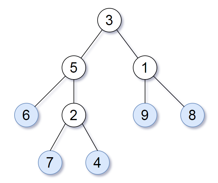
Consider all the leaves of a binary tree. From left to right order, the values of those leaves form a leaf value sequence.

For example, in the given tree above, the leaf value sequence is (6, 7, 4, 9, 8).

Two binary trees are considered leaf-similar if their leaf value sequence is the same.

Return true if and only if the two given trees with head nodes root1 and root2 are leaf-similar.

Note:

• Both of the given trees will have between 1 and 100 nodes.

Problem

Given a m x n grid filled with non-negative numbers, find a path from top left to bottom right which minimizes the sum of all numbers along its path.

Note: You can only move either down or right at any point in time.

Example

1
2
3
4
5
6
7
8

Input:
[
  [1,3,1],
  [1,5,1],
  [4,2,1]
]
Output: 7
Explanation: Because the path 1→3→1→1→1 minimizes the sum.

Problem

Given a collection of intervals, merge all overlapping intervals.

Examples

1
2
3

Input: [[1,3],[2,6],[8,10],[15,18]]
Output: [[1,6],[8,10],[15,18]]
Explanation: Since intervals [1,3] and [2,6] overlaps, merge them into [1,6].

1
2
3

Input: [[1,4],[4,5]]
Output: [[1,5]]
Explanation: Intervals [1,4] and [4,5] are considered overlapping.

Boundary Conditions

The World of Many Weak Features

Often we have many relatively weak features to apply to a classification problem.

In Text classification problems, we often have the frequency of each word in documents of positive and negative classes: e.g. the frequency of sale in spam and real email.

Bayesian Classifiers

To classify a vector $X = (x_1, …, x_n)$ into one of $m$ classes, we can use Bayes Theorem:
$$
p(C_i|X)=\frac{p(C^i)p(X|C_i)}{p(X)}
$$
This reduces decisions about the class given the input to the input given the class.

Identifying the Most Probable Class

Argmax is the class with the highest probability:
$$
C(X)=\max_{i=1}^m\frac{p(C_i)p(X|C_i)}{p(X)}=\max_{i=1}^mp(C_i)p(X|C_i)
$$
$p(C_i)$ is the prior probability of class $i$

$p(X)$ is the probability of seeing input $X$ over all classes. This is dicey, but can be ignored for classification because it constant.

Independence and Naive Bayes

What is $p(X|C)$, where $X$ is a complex feature vector?

If $(a, b)$ are independent, then $p(ab) = p(a)p(b)$ this calculation is much simpler than factoring in correlations and interactions of multiple factors, but:

What’s the probability of having two size 9 feet?

Complete Naive Bayes Formulation

We seek the argmax of:
$$
C(X) = \max_{i=i}^mp(C_i)p(X|C_i)=\max_{i=1}^mp(C_i)\Pi_{j=1}^np(x_j|C_i)
$$
Multiplying many probabilities is bad, so:
$$
C(X)=\max_{i=1}^m(\log(p(C_i)) + \sum_{j=1}^n\log(p(x_j|C_i)))
$$

Dealing with Zero Counts

You may never have seen it before, but what is the probability my next word is defenestrate?

Observed counts do not accurately capture the frequency of rare events, for which there is typically a long tail.

Laplace asked: What is the probability the sun will rise tomorrow?

+1 Discounting

Discounting is a statistical technique to adjust counts for yet-as-unseen events. The simplest technique is add one discounting, where we add one to the frequency all outcomes, including unseen. Thus after seeing 5 reds and 3 greens,
$$
p(new-color) = \frac{1}{(5+1)+(3+1)+(0+1)} = \frac{1}{11}
$$

Feature Engineering

Domain-dependent data cleaning is important:

• Z-scores and normalization
• Creating bell-shaped distributions
• Imputing missing values
• Dimension reduction, like SVD
• Explicit incorporation of non-linear combinations like products and ratios

Deep Learning

The hottest area of machine learning today involves large, deep neural network architectures.

Basic Principles of Deep Learning

• That the weight of each edge is a distinct parameter means large networks exploits large training sets.
• The depth of the networks means they can build up hierarchical representations of features: e.g. pixels, edges, regions, objects
• Toolkits like TensorFlow make it easy to build DL models if you have the data

Node Computations

Each node in the network typically computes a nonlinear function Phi(v) of a weighted input sum:
$$
v_j = \beta + \sum_iw_ix_i
$$
The beta term is the bias, the activation in the absence of input.

Many dot products implies matrix multiplication!

Non-Linearity

The logit and RELU functions make good candidates for Phi. Linear function like addition cannot exploit depth, because hidden layers add no power.

Backpropagation

NNs are trained by a stochastic gradient descent-like algorithm, with changes for each training example pushed down to lower levels. The non-linear functions result in a non-convex optimization function, but this generally produces good results.

Word Embeddings

One NN application I have found particularly useful is word2vec, constructing 100 dimensional word representations from text corpora.

The goal is to try to predict missing words by context: We would ** to improve

Thus large volumes of training data can be construction from text without supervision.

Graph Embeddings (DeepWalk)

Networks based on similarity or links define very sparse feature vectors.

Random walks on networks (sequences of vertices) look like sentences (sequences of words).

Thus we can use word2vec to train network representations.

Support Vector Machines

SVMs are an important way to build non-linear classifiers.

They work by seeking maximum margin linear separators between the two classes.

Optimization Problem

Optimize the coefficient size $||w||$ subject to the constraints $y_i(\bold{w} \cdot \bold{x_i} - b)\geq 1$ for all i = 1, …, n.

only a few points touch the boundary of the separating channel. Near-vertical lines are closer than horizontal lines even b +/- 1 are 2 apart, hence minimizing on $||w||$.

SVMs vs. Logistic Regression

Both methods find separating planes, but different ones.

LR values all points, but SVM only the points at the boundary.

Projecting to Higher Dimensions

Adding enough dimensions makes everything linearly separable.

Here $(x, y)\rightarrow (x, y, x^2+y^2)$ does the job.

Efficient solvers like LibSVM are available for this.

Projecting to Higher Dimensions

The non-linearity depends upon how space is projected to higher dimensions. The distance from all $n$ input points to the target creates an n-dimensional feature vector.

Kernal functions give the power to use such features efficiently, without building the $n\times n$ matrix.

Summary

• Linear regression has a beautiful theoretical foundation yet, in practice, this algebraic formulation is generally discarded in favor of faster, more heuristic optimization.
• Linear regression models are, by definition, linear. This provides an opportunity to witness the limitations of such models, as well as develop clever techniques to generalize to other forms.
• Linear regression simultaneously encourages model building with hundreds of variables, and regularization techniques to ensure that most of them will get ignored.

Unification

One of the main ingredients in the inference mechanism is the process of making atomic formulas syntactically equivalent. This process, called unification, is a procedure that take two atomic formulas as input, and either shows how they can be instantiated to identical atoms or, reports a failure.

Informal Introduction

Classification Problems

Often we are given collections of examples labeled by class:

• male/female
• democrat/republican
• spam/non-spam (ham)
• cancer/benign

Classification assigns a babel to an input record.